Introduction#
The optimisation of the Argo array is quite complex to determine in specific regions, where the local ocean dynamic shifts away from standard large scale open ocean. These regions are typically the Boundary Currents where turbulence is more significant than anywhere else, and Polar regions where floats can temporarily evolve under sea-ice. Furthermore, with the development of Argo float recovery initiatives, it becomes more crucial than ever to be able to predict float trajectories with mission parameters that can be modified on-demand remotely.
VirtualFleet aims to help the Argo program to optimise floats deployment and programming.
To do so, the VirtualFleet software provides a user-friendly, high-level, collection of Python modules and functions to make it easy to simulate Argo floats.
The general principle is to customise the behavior of particles in a Lagrangian simulation framework (OceanParcels2019) using output from ocean circulation models.
Simulated cycle#
Although a virtual Argo float is not as complex as a real one, it simulates the typical Argo float cycle with the most important phases:
descent to a a predefined parking depth (phase 0),
free drifting phase at this predefined parking depth (phase 1),
descent to a predefined profiling depth followed by an ascent to surface (phase 2-3),
a free drift at the surface to mimic time for geo-positioning and satellite data transmission (phase 4).
This cycle and the simplified associated mission parameters are illustrated figure 1.
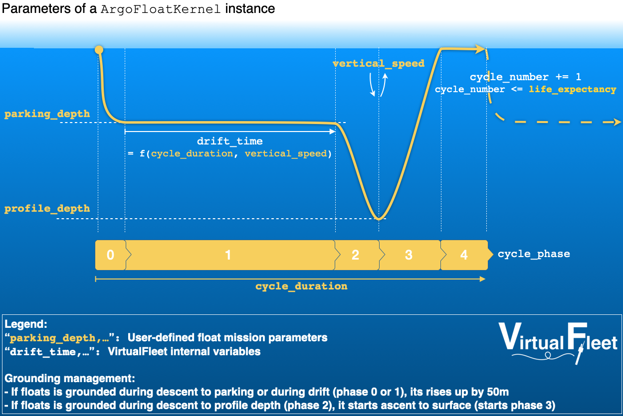
Fig. 1 Schematic of an Argo float cycle in VirtualFleet#
Components#
In the VirtualFleet software:
a virtual float is represented by an
ArgoParticleinstance,a virtual float cycle is encoded by an
ArgoFloatKernel()function,
Furthermore:
a
VirtualFleetinstance represents a fleet of virtual floats, including a deployment plan and the ocean velocity field to transport floats,one use a
VirtualFleetinstance to execute a simulation.
The 3 technical requirements to be able to simulate a virtual fleet are the following:
You will find all details about these requirements, together with the VirtualFleet software helpers to fulfill them in the “Preparation of a simulation” section.
Executing a simulation is explained in the “Running a virtual fleet simulation” section and “Simulation analysis” get you started with the analysis of the results.
References#
The Parcels v2.0 Lagrangian framework: new field interpolation schemes. Delandmeter, P and E van Sebille (2019), Geoscientific Model Development, 12, 3571–3584